
Introduction
Imagine showing a computer a picture of a cat and asking, “Is this a cat, a dog, or a rocket?” Without any prior training on your specific images, the computer answers correctly. This isn’t science fiction—it’s CLIP (Contrastive Language-Image Pre-training), one of OpenAI’s most revolutionary models that bridges the gap between vision and language.
In this comprehensive guide, we’ll walk through CLIP’s architecture, implementation, and inner workings in a way that anyone can understand, even if you’re just starting your journey in AI and machine learning.
Resources:
What Makes CLIP Special?
Traditional image classification models need thousands of labeled examples to recognize new categories. If you want your model to recognize “bicycle,” you need to show it thousands of bicycle images during training. But CLIP works differently—it can recognize objects it has never explicitly been trained on. This is called zero-shot classification.
CLIP achieves this by learning the relationship between images and text descriptions. Instead of learning “this is a cat,” it learns “images that look like this match with text descriptions like ‘a photo of a cat.'”
The Big Picture: How CLIP Works
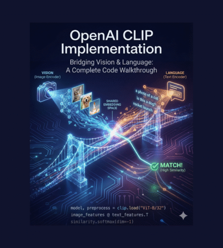
Think of CLIP as having two specialists working together:
- The Vision Specialist (Vision Transformer): Takes an image and converts it into a numerical representation (a vector)
- The Language Specialist (Text Transformer): Takes text descriptions and converts them into numerical representations
These two specialists speak the same “language”—they both create 512-dimensional vectors. By comparing these vectors using simple dot products, CLIP can determine how well an image matches a text description.
Setting Up: Prerequisites
Before diving into the code, let’s understand what you’ll need:
python
# Install required packages
!pip install ftfy regex tqdm
!pip install git+https://github.com/openai/CLIP.git

import numpy as np
import torch
import clip
What these do:
ftfy: Fixes text encoding issuesregex: Handles complex text pattern matchingtqdm: Shows progress barsclip: The main CLIP library
Loading the CLIP Model
python
model, preprocess = clip.load("ViT-B/32")This single line does a lot of heavy lifting. Let’s break it down:
- ViT-B/32: This specifies we’re using a Vision Transformer (ViT) with “Base” size, where images are divided into 32×32 pixel patches
- model: The actual CLIP model with ~151 million parameters
- preprocess: A function that prepares images in the format CLIP expects
Model Specifications
When you load CLIP, you get:
- Input Resolution: 224×224 pixels (all images are resized to this)
- Context Length: 77 tokens (maximum text length)
- Vocab Size: ~49,000 unique tokens
- Embedding Dimension: 512 (the final vector size)
The Vision Pipeline: From Pixels to Vectors
Step 1: Image Preprocessing
python
preprocess(image)
```

This transforms your image through several steps:

1. **Resize to 224×224**: Makes all images the same size
2. **Center Crop**: Focuses on the central part of the image
3. **Convert to RGB**: Ensures consistent color channels
4. **Normalize**: Adjusts pixel values using ImageNet statistics (mean and standard deviation)

Think of preprocessing like formatting a document before sending it to a printer—you need consistent margins, paper size, and orientation.

### Step 2: Patchification (Breaking Images into Pieces)

The Vision Transformer doesn't process the entire image at once. Instead, it:

1. Divides the 224×224 image into 32×32 pixel patches
2. This creates a 7×7 grid = 49 patches (since 224÷32 = 7)
3. Each patch is flattened and converted into a 768-dimensional vector

**Visual Representation:**
```
Original Image (224×224×3)
         ↓
Divided into patches (7×7 grid of 32×32 patches)
         ↓
Each patch → 768-dimensional vector
         ↓
Result: 49 vectors of 768 dimensions each
Step 3: Adding Special Tokens and Position
python
# Add CLS token (classification token)
cls_token = learnable_parameter(768 dimensions)

# Add positional embeddings
positional_embeddings = learnable_table(50 × 768)
# 50 = 49 patches + 1 CLS token
Why do we need these?
- CLS Token: A special “summary” token that learns to represent the entire image. Think of it as the chapter summary at the end of a book.
- Positional Embeddings: These tell the model WHERE each patch is in the image. Without this, the model wouldn’t know if a patch is from the top-left or bottom-right corner.
Step 4: The Transformer Magic
The Vision Transformer consists of 12 layers, each with:
- Multi-Head Attention: Lets each patch “look at” and learn from other patches
- MLP (Multi-Layer Perceptron): Processes information with a pattern: 768 → 3072 → 768 dimensions
- Layer Normalization: Keeps values stable during training
After 12 layers of processing, we extract the vector above the CLS token and project it from 768 to 512 dimensions. This 512-dimensional vector is our image embedding.
The Language Pipeline: From Text to Vectors
Step 1: Tokenization (The Hardest Part!)
Tokenization converts text into numbers. CLIP uses Byte Pair Encoding (BPE), which is like creating a smart dictionary:
python
text = "Hello World!"
tokens = clip.tokenize(text)
# Result: [49406, 3306, 1002, 0, 0, ..., 0, 49407]
#         [START, hello, world, 0s (padding), END]
How BPE Works (Simplified):
- Start with individual characters: “h”, “e”, “l”, “l”, “o”
- Find the most frequent pairs and merge them: “he”, “ll”, “o”
- Repeat until you have a vocabulary of ~49,000 tokens
- Some words are single tokens, others are split into sub-words
Example with Emoji:
python
text = "🧠"  # Brain emoji
# UTF-8 encoding: 4 bytes
# BPE splits into 2 tokens: [8792, 510]
The beauty of BPE is it can handle ANY text, even words it’s never seen, by breaking them into smaller pieces.
Step 2: Token Embedding
python
token_embedding_table = learnable_matrix(49408 × 512)
# 49408 = vocabulary size
# 512 = embedding dimension

# For token ID 3306 (hello)
embedding = token_embedding_table[3306]  # Gets a 512-dim vector
Each token ID gets converted to a 512-dimensional vector by looking it up in this table.
Step 3: Adding Positional Information
python
positional_embedding_table = learnable_matrix(77 × 512)
# 77 = context length

# Add position info to each token
final_embeddings = token_embeddings + positional_embeddings
This tells the model the ORDER of words. “Dog bites man” vs “Man bites dog” have the same words but different meanings!
Step 4: Text Transformer
Similar to the Vision Transformer, but with:
- Causal Attention Mask: Each word can only “see” previous words, not future ones
- 12 transformer layers
- Projects to 512 dimensions
Extracting the Final Vector: After processing, CLIP takes the vector at the position of the [END] token. This vector represents the entire sentence’s meaning.
Bringing It Together: Calculating Similarity
Now we have:
- Image embedding: 512-dimensional vector
- Text embedding: 512-dimensional vector
Step 1: Normalization
python
image_features /= image_features.norm(dim=-1, keepdim=True)
text_features /= text_features.norm(dim=-1, keepdim=True)
This makes all vectors have a length of 1.0 (unit vectors). Why? So we’re comparing DIRECTION, not magnitude.
Analogy: Think of compass directions. Whether you walk 1 mile north or 10 miles north, you’re still going “north.” Normalization focuses on the direction (north) rather than the distance (1 vs 10 miles).
Step 2: Dot Product (Similarity Score)
python
similarity = image_features @ text_features.T
```

The `@` operator performs matrix multiplication, which calculates dot products between all image-text pairs.

**What's a dot product?**
```
Vector A = [1, 2, 3]
Vector B = [4, 5, 6]

Dot Product = (1×4) + (2×5) + (3×6) = 4 + 10 + 18 = 32
For normalized vectors:
- Dot product = 1.0 means vectors point in the same direction (very similar)
- Dot product = 0.0 means vectors are perpendicular (unrelated)
- Dot product = -1.0 means vectors point in opposite directions (opposite meanings)
Step 3: Softmax for Probabilities
python
probabilities = (100.0 * similarity).softmax(dim=-1)Multiplying by 100 amplifies differences, then softmax converts scores to probabilities that sum to 1.0.
Zero-Shot Classification: The Magic Trick
Here’s where CLIP shines. To classify an image without training:
Method 1: Simple Template
python
# For CIFAR-100 with 100 classes
texts = [f"This is a photo of a {label}" for label in classes]
# Creates: "This is a photo of a cat", "This is a photo of a dog", ...

# Encode all 100 text descriptions
text_features = model.encode_text(texts)  # Shape: (100, 512)

# Encode the image
image_feature = model.encode_image(image)  # Shape: (1, 512)

# Calculate similarities
similarities = image_feature @ text_features.T  # Shape: (1, 100)

# Highest similarity = predicted class
predicted_class = similarities.argmax()
Why This Works:
Think of it like this: You’ve created 100 “direction arrows” (one for each class). When you get a new image, you see which direction arrow it points closest to. No training needed!
Method 2: Ensemble with Multiple Templates (Better Results!)
python
templates = [
    "a photo of a {}",
    "a bad photo of a {}",
    "a photo of many {}",
    "a sculpture of a {}",
    "a photo of the large {}",
    # ... 75 more templates
]

# For each class, create 80 different descriptions
for class_name in classes:
    descriptions = [template.format(class_name) for template in templates]
    embeddings = model.encode_text(descriptions)  # Shape: (80, 512)

    # Average all 80 embeddings
    class_embedding = embeddings.mean(dim=0)  # Shape: (512,)

    # Normalize again
    class_embedding /= class_embedding.norm()
```

**Why Ensemble Works Better:**

Instead of one description, you're using 80 different ways to describe the same thing. It's like asking 80 people to describe a cat, then averaging their descriptions—you get a more robust representation that captures various aspects and viewpoints.

This improved ImageNet accuracy by 1.5% for ViT-B/32!

## The Ad-Hoc Classifier: A Clever Insight

Here's a mind-bending insight: When you create text embeddings for classes, you're actually constructing the weights of a classification layer on-the-fly!

**Traditional Classifier:**
```
Image (512-dim) → Linear Layer (512 × 1000 weights) → 1000 class scores
                   ↑
                   Learned during training
```

**CLIP's Zero-Shot Classifier:**
```
Image (512-dim) → Dot Products → 1000 class scores
                   ↑
                   Weights = Text embeddings (1000 × 512)
                   Created instantly from class names!
```

**Visual Representation:**
```
Image Vector: [0.1, 0.5, 0.3, ..., 0.8]  (512 values)
              ×
Class Vectors:
  "cat":  [0.2, 0.4, 0.1, ..., 0.7]
  "dog":  [0.3, 0.1, 0.5, ..., 0.2]
  "car":  [0.1, 0.8, 0.2, ..., 0.4]
  ...
  =
Similarity Scores: [0.85, 0.42, 0.31, ...]
Each dot product is equivalent to one neuron in a classification layer!
Practical Implementation: Complete Example
Let’s put everything together with a complete example:
python
import torch
import clip
from PIL import Image

# 1. Load model
device = "cuda" if torch.cuda.is_available() else "cpu"
model, preprocess = clip.load("ViT-B/32", device=device)

# 2. Prepare image
image = Image.open("your_image.jpg")
image_input = preprocess(image).unsqueeze(0).to(device)

# 3. Prepare text descriptions
text_descriptions = [
    "a photo of a cat",
    "a photo of a dog",
    "a photo of a car"
]
text_inputs = clip.tokenize(text_descriptions).to(device)

# 4. Get embeddings
with torch.no_grad():
    image_features = model.encode_image(image_input)
    text_features = model.encode_text(text_inputs)

    # Normalize
    image_features /= image_features.norm(dim=-1, keepdim=True)
    text_features /= text_features.norm(dim=-1, keepdim=True)

    # Calculate similarity
    similarity = (100.0 * image_features @ text_features.T).softmax(dim=-1)

# 5. Get prediction
values, indices = similarity[0].topk(3)
print("\nPredictions:")
for value, index in zip(values, indices):
    print(f"{text_descriptions[index]:>20s}: {100 * value.item():.2f}%")
Key Concepts to Remember
1. Embeddings are Directions in Space
Think of embeddings as GPS coordinates. Similar concepts have coordinates close together, different concepts are far apart.
2. Normalization Focuses on Direction
By making all vectors length 1, we compare “where they’re pointing” not “how far they go.”
3. Dot Product Measures Similarity
- High dot product (close to 1) = similar meaning
- Low dot product (close to 0) = different meanings
4. Transformers Allow Interactions
Each part of the image (or text) can “communicate” with other parts to build understanding.
5. Positional Information Matters
Without positional embeddings, the model wouldn’t know the ORDER of words or LOCATION of image patches.
Common Pitfalls and Tips
Pitfall 1: Not Normalizing Features
python
# Wrong - will give poor results
similarity = image_features @ text_features.T

# Correct
image_features /= image_features.norm(dim=-1, keepdim=True)
text_features /= text_features.norm(dim=-1, keepdim=True)
similarity = image_features @ text_features.T
Pitfall 2: Forgetting to Preprocess Images
python
# Wrong
image_input = torch.tensor(np.array(image))

# Correct
image_input = preprocess(image).unsqueeze(0)
Pitfall 3: Poor Text Descriptions
python
# Less effective
texts = ["cat", "dog", "car"]

# More effective
texts = ["a photo of a cat", "a photo of a dog", "a photo of a car"]
Performance Insights
CLIP’s performance on ImageNet:
- Top-1 Accuracy: ~55% (zero-shot)
- Top-5 Accuracy: ~83.4% (zero-shot)
This means:
- The correct class is in the top prediction 55% of the time
- The correct class is in the top 5 predictions 83.4% of the time
For comparison, traditional supervised models need thousands of ImageNet training examples to reach ~76% top-1 accuracy.
Advanced Topics
Linear Probe (Optional Training)
Instead of zero-shot, you can train a simple classifier on CLIP’s features:
python
# Extract features for training set
train_features = []
train_labels = []

for image, label in training_dataset:
    with torch.no_grad():
        features = model.encode_image(preprocess(image))
        features /= features.norm()
    train_features.append(features)
    train_labels.append(label)

# Train logistic regression
from sklearn.linear_model import LogisticRegression
classifier = LogisticRegression()
classifier.fit(train_features, train_labels)

# Test
accuracy = classifier.score(test_features, test_labels)
This typically gives better results than zero-shot because the classifier learns from your specific dataset.
Conclusion
CLIP represents a paradigm shift in computer vision. Instead of training separate models for each task, CLIP learns a shared space where images and text can be directly compared. This enables:
- Zero-shot classification: Classify without training
- Flexibility: Add new classes by simply adding text descriptions
- Multimodal understanding: Bridge vision and language naturally
The key innovations are:
- Joint training on images and text
- Contrastive learning to align similar pairs
- Large-scale training on 400 million image-text pairs
- Flexible architecture using Vision and Text Transformers
Next Steps
To deepen your understanding:
- Experiment: Try CLIP on your own images and text
- Read the paper: “Learning Transferable Visual Models From Natural Language Supervision”
- Explore variants: Check out CLIP variants like OpenCLIP, BLIP, etc.
- Build applications: Use CLIP for image search, content moderation, or creative tools
Remember: The best way to learn is by doing. Start with the simple example above, then gradually explore more complex use cases. Good luck on your CLIP journey!
Comments